
I’m a Research Fellow at the Flatiron Institute, Simons Foundation, working jointly at the Center for Computational Neuroscience and the Center for Computational Mathematics. I did a Ph.D. in Data Science at the Center for Data Scienceat New York University, advised by Eero Simoncelli. Here is my thesis. I studied Solid State Physics for my bachelor’s and Psychology for my master’s.
I’m broadly interested in vision and more specifically in probability densities of natural images. I have studied these densities from various angles: learning them from data, understanding and evaluating the learned models, and utilizing them for real-world problems. These areas are closely intertwined: understanding a learned model can inspire the design of better and more efficient ones. Conversely, better performance can hint at something meaningful the model has captured about the underlying data structures. I enjoy studying these complementary perspectives and seeing how they inform one another through careful and controlled scientific experimentation.
Learning Image Density Models from Data
Learning and sampling from a density implicit in a denoiser
Before deep learning, one of the major approches to solve Gaussian denoising problem (as well as other inverse problems) was to assume a prior over the space of images (e.g. Gaussian, Union of subspaces, Markov random fields) and then estimate a solution in a Bayesian framework. The denoiser performance depended on how well this prior approximated the “true” images density. Designing image priors, however, is not trivial and progress relied on empirical findings about image structures – like spectral, sparsity, locality – which led to a steady but slow improvments.
Deep learning revolution upended this trend. We gained access to computrational tools to learn, with unprecedented success, complex high-dimensional mappings for tasks such as denoising, segmentation, classification, etc. without assuming a prior. Yet this phenomenal performance raises a question: what is the prior that the learned mapping impliciltly relies on? …
Click here to see a summary
Remarkably, in the case of Gaussian denoising, the relationship between the denoising mapping and the prior is exact and explicit, thanks to a classical statistics result [Robin 1956, Miyasawa 1961]:
\[\hat{x}(y) = y + \sigma^2 \nabla_y \log p (y)\]See Raphan 2011 for proof.
A Deep Neural Network (DNN) denoiser, \(\hat{x}_{\theta}(y)\), hence, computes the score (gradient of the log probablity) of noisy images, \(y\). When the DNN denoiser learns to solve the problem at all nosie levels, it could be used in an iterative coarse-to-fine gradient ascent algorithm to sample from the density embedded in the denoiser. We introduced this algorithm in the paper below. Its core idea is similar and concurrent to what became known as diffusion models.
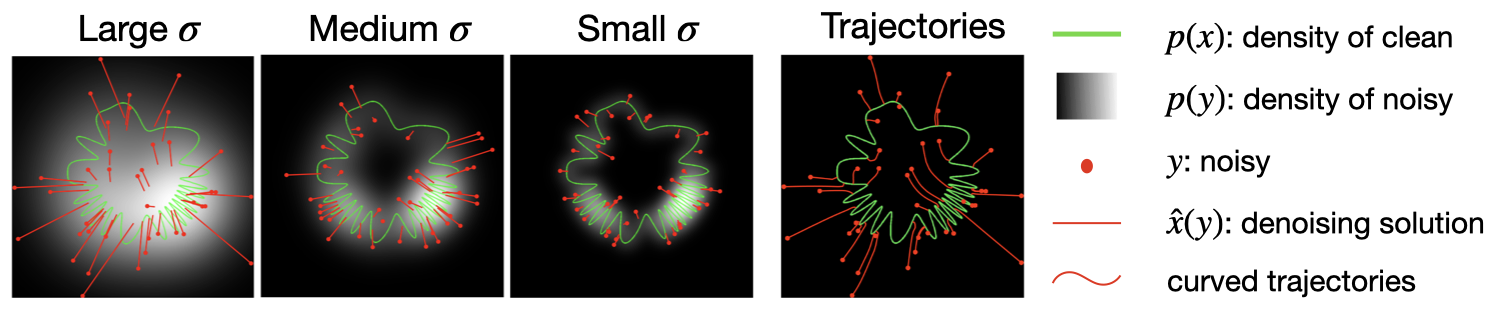
A two-dimensional simulation of the sampler. Right panel shows trajectory of our iterative coarse-to-fine sampling algorithm, starting from the same initial values y (red points) of the first panel. The trajectories are curved, and always arrive at solutions on the signal manifold.
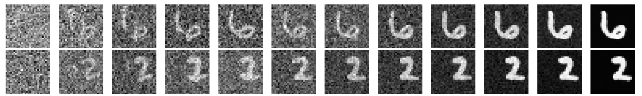
Example sampling trajectory for a model trained on MNIST images.
Two key properties of our algorithm are that 1) the denoiser is noise-level-blind – it does not take as input \(\sigma\). This allows an adaptive noise schedule during sampling, where the step size depends on the noise amplitute estimated by the model. 2) The injected noise at each iteration can be tuned to steer the sampling trajectory toward lower- or higher-probability regions of the distribution, with guaranteed convergence.
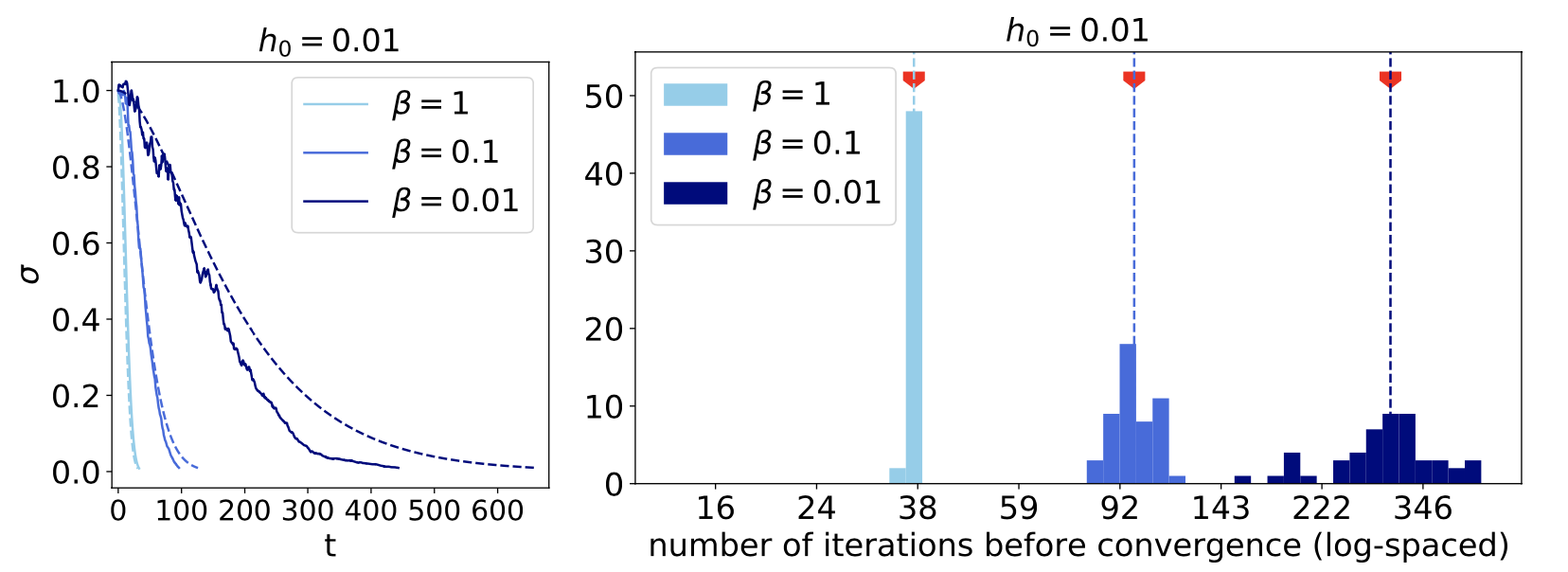
Left: Noise level of the sample as a function of iteration in synthesis, shown for 3 levels of injected noise. More noise (smaller beta) results in more steps. Right: Adaptive algorithm results in varying number of steps for different samples.
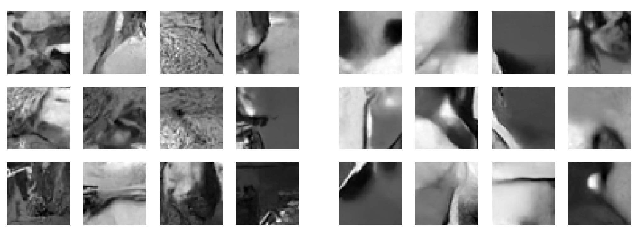
More noise during synthesis results in higher probability images (right panel) by escaping smaller maxima (model trained on patches of grayscale images).
Reference:
ZK & Simoncelli, Solving linear inverse problems using the prior implicit in a denoiser. arXiv, July 2020. PDF | Project page
Later published as: ZK & Simoncelli, Stochastic Solutions for Linear Inverse Problems using the Prior Implicit in a Denoiser. NeurIPS, 2021. PDF
Learning normalized image density rather than the score
Can the embeded prior in a denoiser be made more explict by predicting the energy (\(-\log p\)) rather than the score (\(\nabla \log p\))?
Click here to see a summary
There are two main problems to tackle to make this happen: 1) finding the right architecture and 2) normalizing the density. Neither of these problems exit for score models. Architecures have been refined, through a collective effort, to have the right inductive biases. This evolution has not happened for energy models, putting them at a considerable disadvange. Additionally, in score models, the normalizing factor is eliminated thanks to the gradient. In the paper below, we introduced two simple tricks to overcome these two issues and learn \(\log p\) directly.
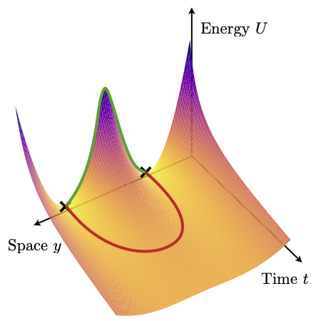
First, we showed that score model architetures can be re-purposed for energy models, by setting the energy to be
\[U_{\theta}(y, t) = \frac{1}{2} \langle y , s_{\theta}(y,t) \rangle\]Second, to get the normalization factor right (up to a global constant), we add a regularization term to the loss function that gaurantees the diffusion equation hold across time (noise levels).
\[\ell_{\rm TSM}(\theta,t) = \mathbb{E}_{x,y} \left[{ \left( {\partial_t U_{\theta}(y,t) - \frac{d}{2t} + \frac{\Vert{y-x}\Vert^2} {2t^2}} \right)^2}\right]\]In effect, minimizing this term ties together the normalization factors of individual \(p(y,t)\). Since the diffused density models are tied together, after training, we can set the normalization factor of \(p(y,t=0)\) by analytcically computing it for \(p(y,t \to \infty)\) (Standard Gaussian) and then transferring it to \(p(x)\).
These two changes do not deteriorate denoisnig performance. This implies the minimizers of the two terms in the dual loss do not fight but reinfornce one another. A model trained using these two tricks returns \(\log p(x)\) in only one forward pass: 1000 times faster than cumbersome computation using a score model.
A good energy model assigns low energy to in-distribution images. We test this on a model trained on ImageNet and show that \(-\log p(x)\) are within the state-of-the-art range.
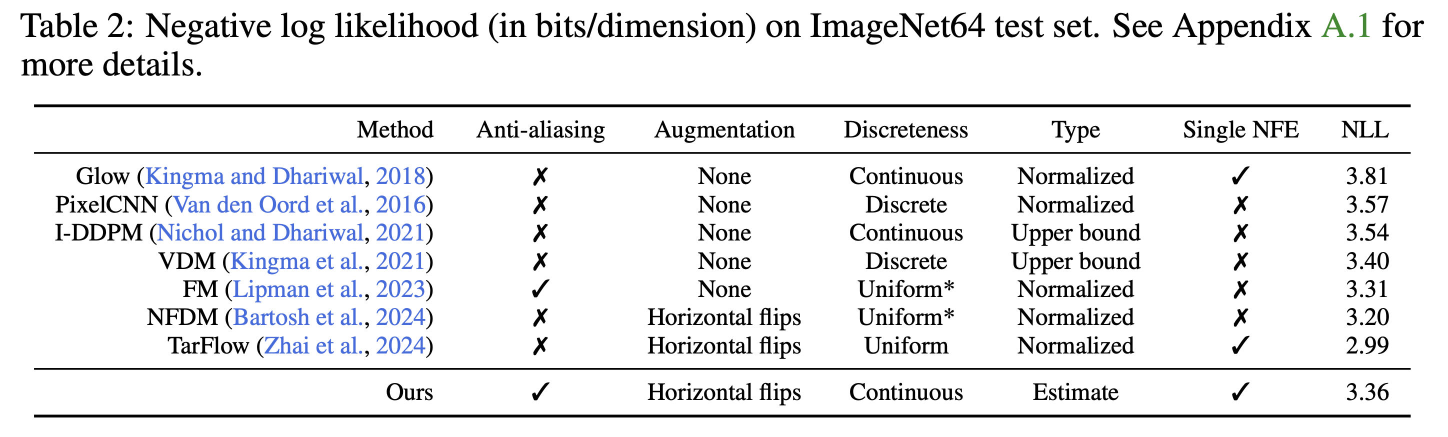
A nice consequence of having direct access to \(\log p(x)\) is that we can now explore image probabilies and study how they relate to image structrues. A surprising (even shocking!) observation is the unbelievably vast range of natural image probabilities. Unlike the common assumption about image distributions, images vary in their probability by a factor of \(10^{14,000}\) (no concentration!). This implies that rare events in the space of images are not so rare when you think about probabilty mass: the volume of the level sets of log probabilties has to be proportional to the inverse of $\log p(x)$. There are many more low probability images than high probability ones.
Additionally, there is a perceptual component strongly tied to the probablity of an image: high probablity images contain more flat regions while low probability images contain lots of details and smaller features which makes them less denoisable.
Histogram of log probabilities of images in the ImageNet dataset. Color-coded arrows indicate values for the example images on the right.
Reference:
Guth, ZK & Simoncelli, Learning normalized image densities via dual score matching. NeurIPS, 2025 PDF
Understanding and Evaluating Learned Density Models
Deep neural networks have grown increasingly complex and deep, while our understanding of them remains comparatively shallow. Why should we try to understand them? Aside from the intrinsic satisfaction of figuring things out, a deeper understanding is essential for evaluating these learned models. In the context of density learning, assessing how “good” a model really begs two questions: 1) How well does it generalize? 2) How accurately does it approximate the true density? Answering these requires knowing where and how such models fail—insight that, in turn, comes from studying why they succeed where they do. I approach these questions through scientific experimentation: explore the data, form hypotheses, and test them under controlled conditions. I believe this mindset suits modern models well. After all, they have evolved through an accelerated process of “natural selection”—only the most effective architectures have survived—making today’s networks far too complex to be fully understood through a purely reductionist, bottom-up theoretical approach.
Generalization in diffusion models
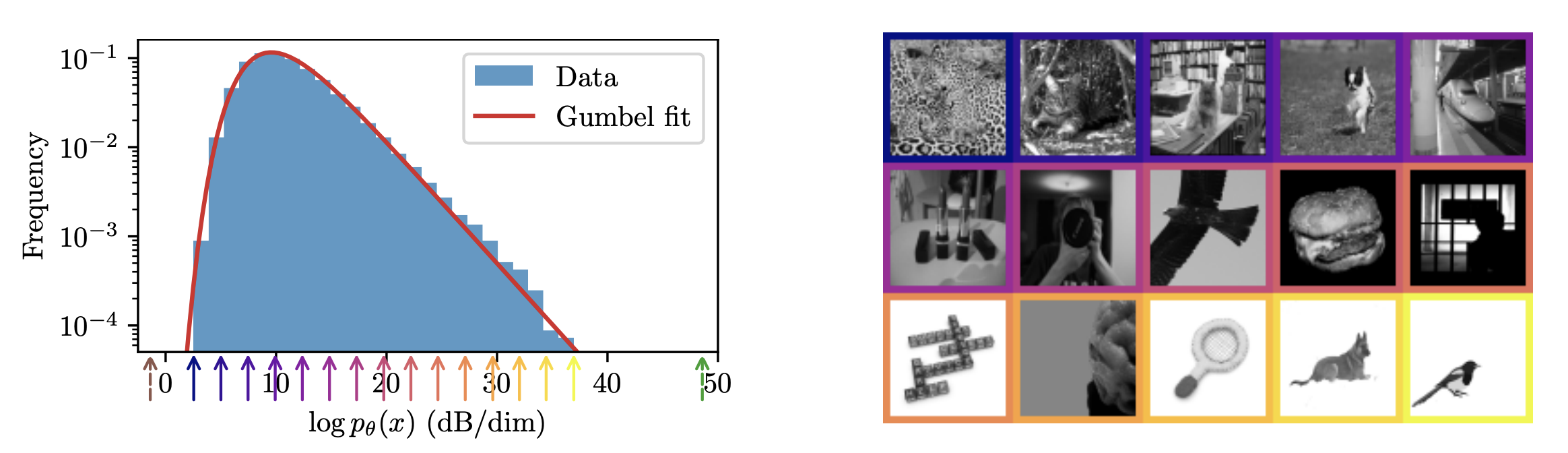
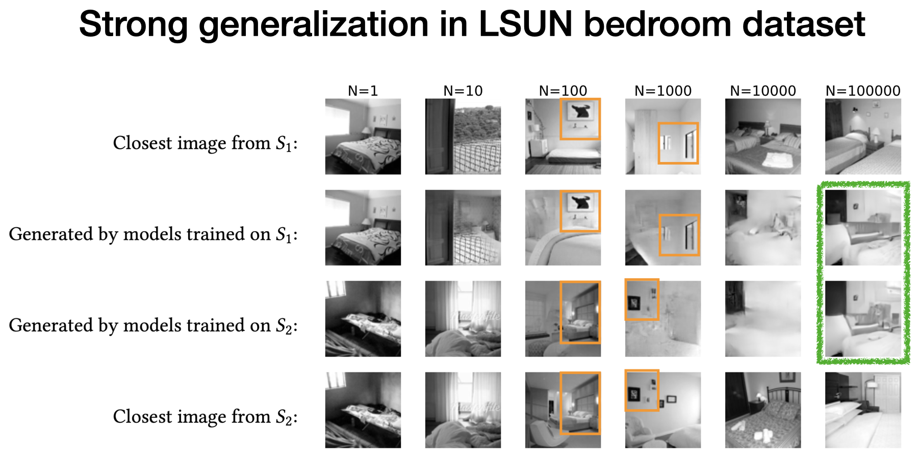
A “good” density model learned from data, does not merely memorize the training set (i.e. the empirical density) but generalizes beyond that. In the paper below, we showed that denoisers used in diffusion models enter a strong generalization phase with finite data, despite the curse of dimensionality …
Click here to see a summary
Convolutional neural net denoisers memorize the training set of very small size. With larger training set, they enter a transition phase in which they either memorize and combine patches of the training exmaples, or return low quality samples. Eventually, they enter a generalization regime in which the two models generate almost the same images if initialize at the same sample (and match the injected iteration noise). This shows that the learned mapping across noise levels becomes independent from the individual images in the training set. In other words, model variance tends to zero.
Refrence
ZK, Guth, Simoncelli, Mallat, Generalization in diffusion models arises from geometry-adaptive harmonic representations. ICLR, 2024 (Best paper award & oral).
PDF | Project page
Denoising is a soft projection on an adaptive basis
Classical denoising heavily relied on designing transformations in which the image representation was sparse. Many of these denoisers worked in three stages: 1) transform the noisy image where noise and image are separable, 2) apply a shrinkage function (soft projection) to suppress the noise, and 3) transform back to pixel space. To maximally preserve the image and remove noise, the image represention in the transformed space shoud be as sparse and compact as possible. But, due to computataional limitations, these transformations were often linear (e.g. Fourier, Wavelet), so failed to fully harvest the intrinsic low-dimensionality of images. Deep neural network denoisers are many times more capable than their classical predecessors. But how do they work? What is the transformation they learn from data? …
Click here to see a summary
To analyze and understand how deep net denoisers work we drew on the insight from the classical literature. In the paper below, we showed that locally-linear DNN denosiers can be described as soft projection (shrinkage) in a sparse basis. What makes them so powerful is that the basis is adaptive to the underlying image, thanks to the nonlinearities of the mapping. The adaptive basis can be exposed by Singular Value Decompotion (SVD) of the Jacobian (\(A_y\)) of the denoising mapping w.r.t. the noisy input. The top singular vectors span the signal subpace which can be interpreted as the tangent plane to the (blurred) image manifold at clean image point.
\[\hat{x}(y) = A_y y = USV^T y = \Sigma_{i =1} ^N s_i (V_i^T y) U_i .\] 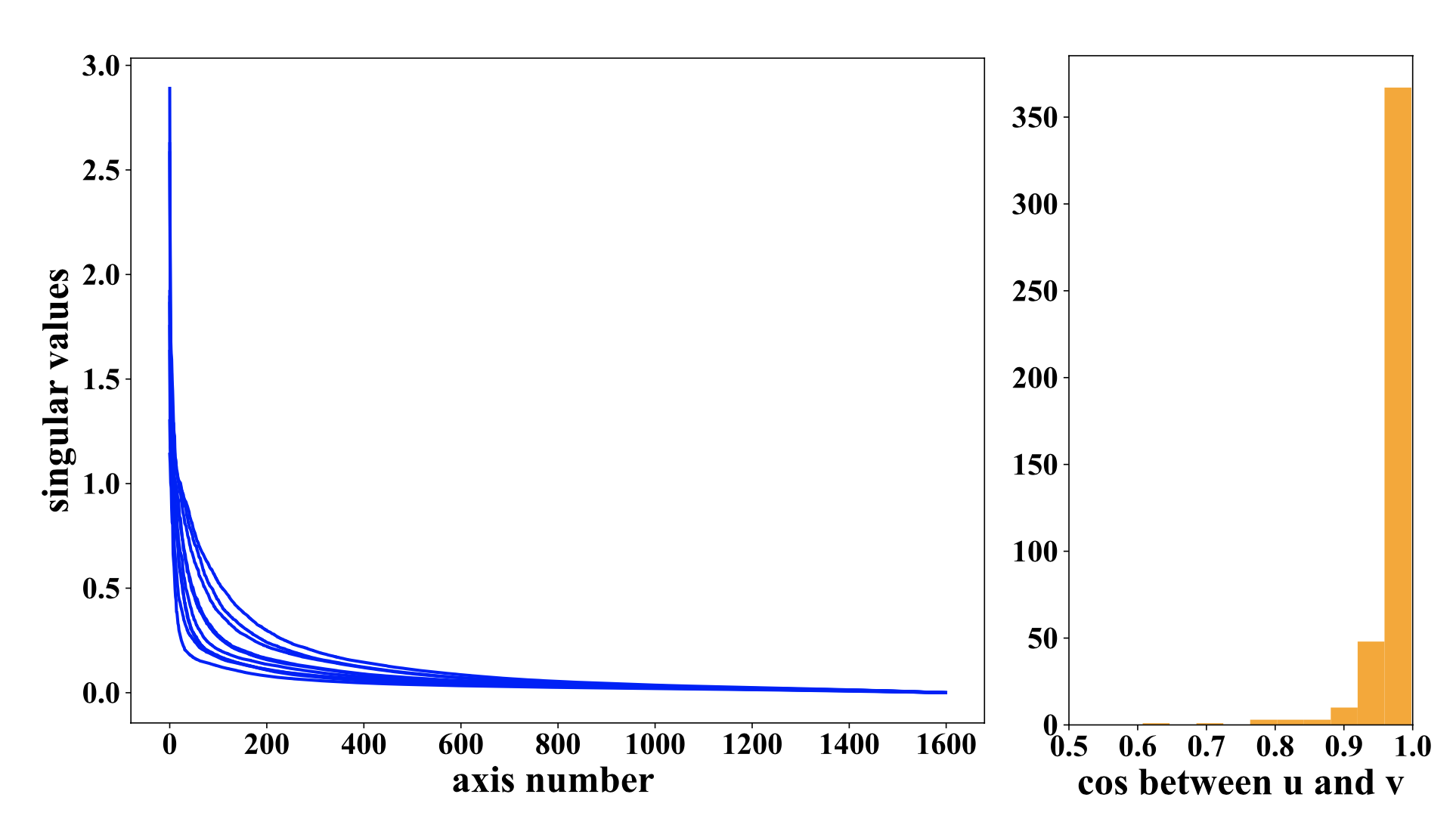
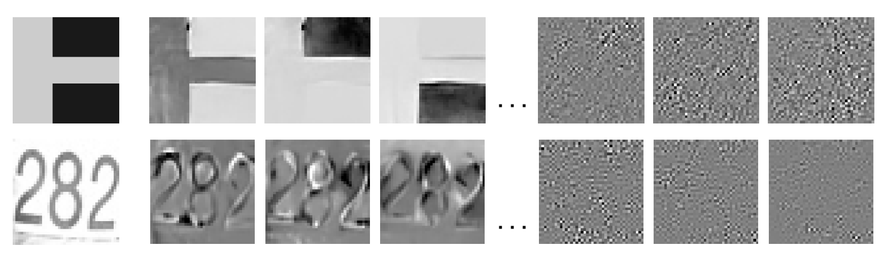
Left: Fast decay of singular values shows that the adaptive basis is very sparse for the input image. Middle: The histogram shows that the Jacobian is almost symmetric. So, the network implements a soft projection onto a basis adaptive to the input. Right: Top singular vectores capture image features which will be preserved and bottom singular vectors are noise which will be supressed.
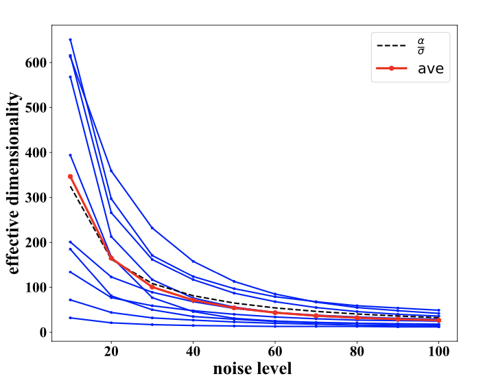
Dimensionality of the subspace is also adaptive and depends on the noise level on the input image. At higher noise levels, fewer signal dimensions can survive the noise. Empirically, dimensionality drops differently for different images, but on average it drops proportional to the inverse of noise level. (See paper for results that shows the subspaces at higher noise levels are nested within subsapces with lower noise levels).
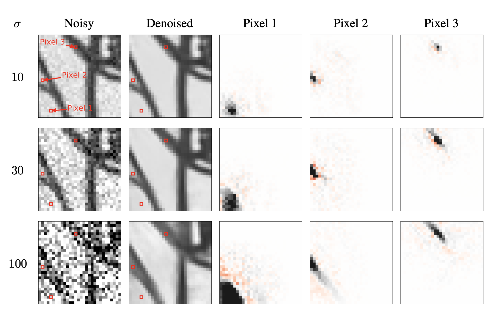
In addition to analysizing the column space of the Jacobian, we also analyzed its row space. Interestingly, we could interpet the DNN denoising mapping as an adaptive filtering procedure in pixel domain, which ties it to another way of formulating denoising in classical signal processing literture (see this review paper). Here, a pixel is estimated by a weighted average of neighboring pixel. The neighborhood weights are daptive to both the noise level and the underlying image structure.
Reference:
Mohan*, ZK*, Simoncelli & Fernandez-Granda, Robust And Interpretable Blind Image Denoising Via Bias-Free Convolutional Neural Networks. ICLR, 2020.
PDF | Project page | Code
* denotes equal contribution
DNN denoisers learn Geometry-adaptive harmonic bases (GAHB)
We made the idea of soft projection in an adaptive basis more precise in the paper below…
Click here to see a summary
Investiagting the denoising mapping in the case of synthetic images where we know the optimal solution reveals that the adpative bases can be characterize with two classes of harmonics: one-dimensional oscilating patterns along the contours and two-dimensional oscillating patterns in the flat backgrounds.
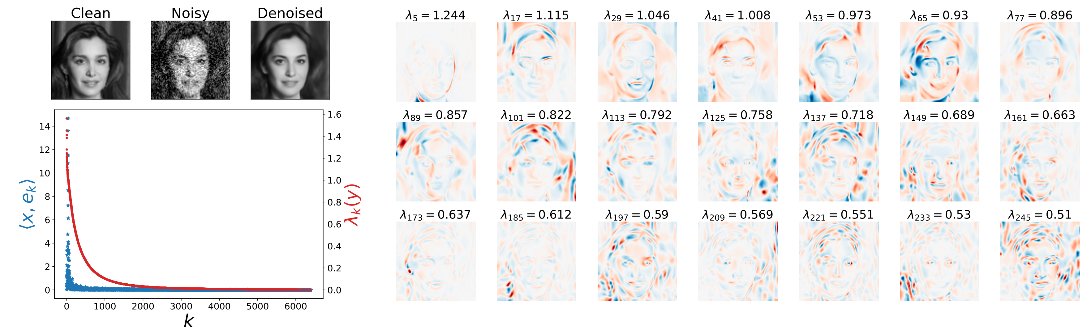
Fast decay of eigen values, and top eigen vectors obtained from the Jacobian of a model trained on CelebA dataset, evaluated at the shown noisy image. We observe 1-D and 2-D oscillating patterns with increasing frequency as a function of eigen value.
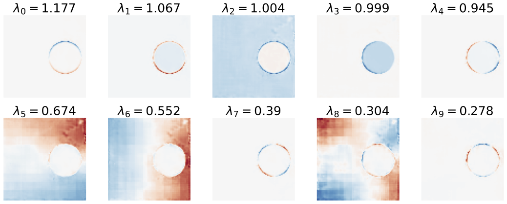
Top eigen vectors of of the Jacobian obtained from a model trained on disc images, evaluated at a slightly noisy disc image. The top eigen vectors span the tangent plane of the 5-dimensional synthesis image manifold, evaluated at one noisy image. The next five eigen values are not zero, which results in a sub-optiml denoising MSE. The network fails to lean the optimal solution due to its preference for GAHBs.
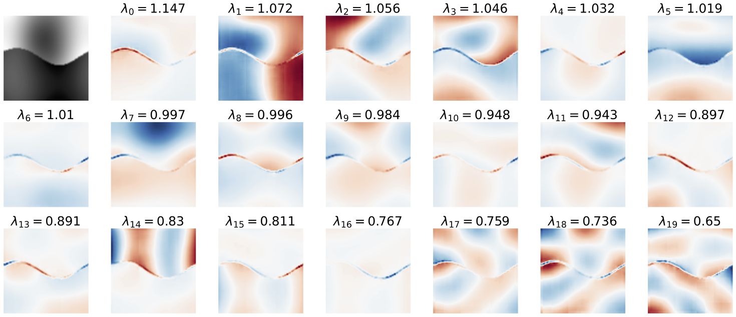
Top eigen vectors of of the Jacobian obtained from a model trained on synthetic images (C-alpha), evaluated at a noisy image. For this class of images, the optimal densoising is obtain within a GAHBs basis. The model learns the optimal solution (see paper for results).
From a mechanistic perspective, the harmanics arise from the convolutional layers. However, these harmonics are way more sophisticated than their precedator, the Fourier basis (weiner filter), due to the non-linearities of the network. Understanding the exact relationship between the GAHBs and the cascade of operations in the network remains to be understood.
Refrence
ZK, Guth, Simoncelli, Mallat, Generalization in diffusion models arises from geometry-adaptive harmonic representations. ICLR, 2024 (Best paper award & oral).
PDF | Project page
Conditional locality of image densities
We showed that diffusion models can overcome the curse of dimensionality and generalize beyond the training set. But how do they achieve this feat? What are the inductive biases that lead to learning the score? How can they learn a high dimensionality density with finite data? In the paper below, we showed that one property of the image densities that’s leverged by the network is the locality of the conditional densities …
Click here to see a summary
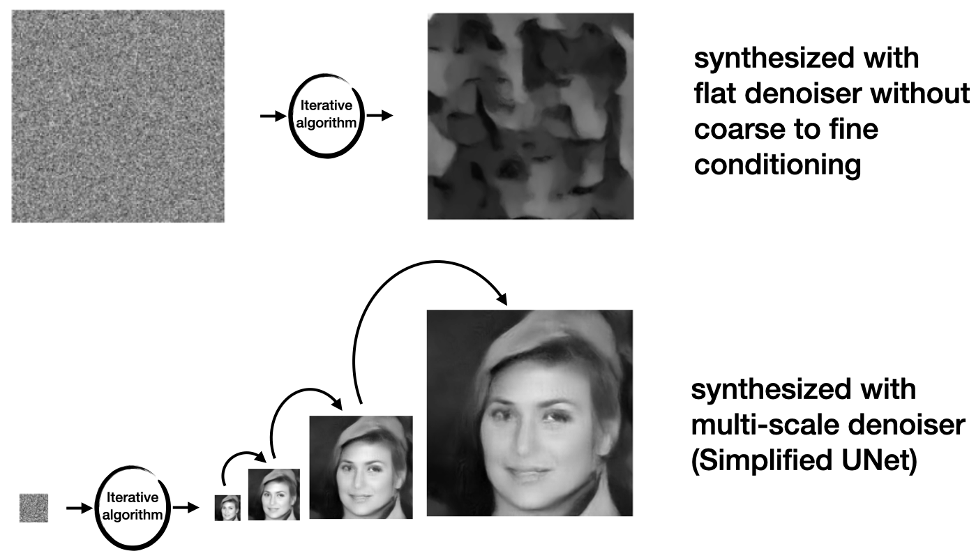
To understand this, we need to open the black box of the DNN denoisers to understand how it works. We took a step in this direction by studying a somewhat simplified UNet architecture. How did we modify the UNet without hurting its performace? We replaced its encoder path with a multi-scale wavelet transform (Haar filter more specfically). It is simply a linear orthogonal transform (\(W\)) which is implemented by only 4 convolutional filters: three of them extract the details,\(\bar{x_j}\), (vertical, horizontal, diagonal differences) and one holds on to the low-resolution coarser content (2x2 averaging). We apply the same 4 filters on the low-resolution image, and keep repeating it to create mutiple blocks. \(j\) denotes depth of the scale (\(j=0\) is the input level, and \(j=J\) is the deepest scale - the bottom block). Using this representation gaurantees that different scales do not overlap, making the model more analyzable.
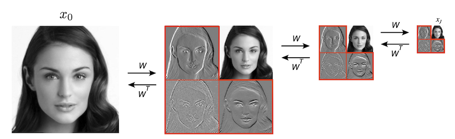
Multi-scale wavelet decomposition of a clean image. This cascade coefficients is used as a substitute for the encoding path of a UNet.
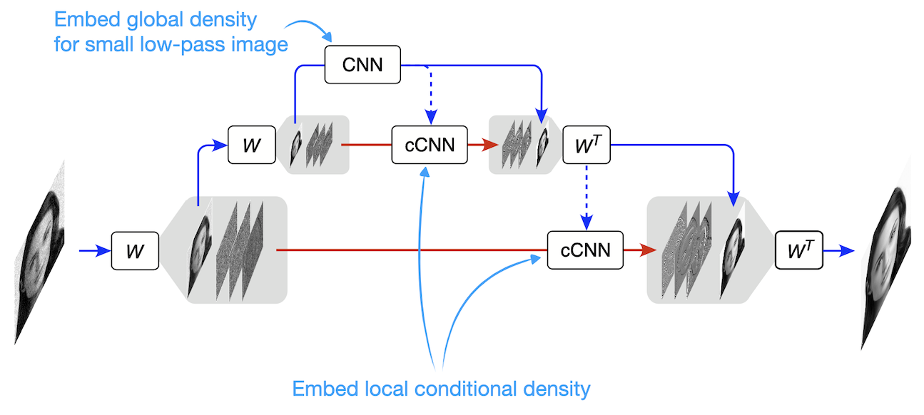
A simplified UNet (upside-down) with a linear encoder path. The encoder consists of a multi-scale wavelet decomposition.
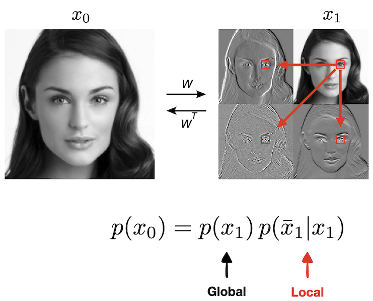
We hypothesized that the UNet overcomes the curse of dimensionality by factorizing the density, \(p(x)\), into a series of lower-dimensional conditional densities. It learns a density of the low-dimensional lowest resolution image, \(p(x_J)\),which captures long range global dependencies. The location information is preserved thanks to the the zero-padding boundary handling that breaks translation equivariance. For the details it learns low-dimensional density of details conditioned on the coarser from the previous block.
But does it make sense to assume the conditional densities are low-dimensional?! The answer is yes! The reduction in dimensionality comes from the conditional-locality of the details density. In other words, \(p(\bar{x_j})\) is not necessarily low-dimensional, but \(p(\bar{x_j} | x_j)\) is: knowing the coarser structure in the image (e.g. blurred outline of a face), we only need a small neighborhood around a pixel to denoise it (or add details). In other words, we are assuming a hierarchical markov property over the details values, and our experiments show that this assumption is aligned with true data structure. We tested this hypothesis by making the Receptive Field (RF) of the decoder blocks as small as \(9 \times 9\) for input images of size \(320 \times 320\) and observed almost no reduction of performance!
Conditioning on a small neighborhood of the low-resolution image, the density over the details can be model by a Markov Random Field, where only dependencies on a small neighborhood are needed.
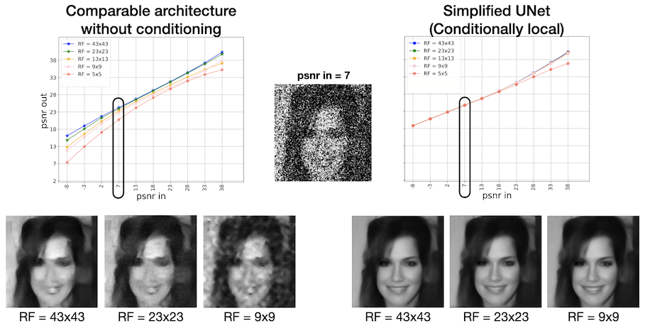
This model can be used to generate images, like a UNet. For comparison, we show a sample generated from a model without coarse-to-fine conditioning with comparable number of parameters. These results show that we can reduce the number of parameters drastically if the architecture leverges structure in the image correctly.
ZK, Guth, Mallat, Simoncelli, Learning multi-scale local conditional probability models of images. ICLR, 2023 (Oral).
PDF | Project page
Unsupervised representation learning via denoising
Diffusion models learn probability densities by estimating the score with a neural network trained to denoise. What kind of representation arises within these networks, and how does this relate to the learned density? In the paper below, we show that a fully unsupervised notion of semantic similarity arises from the task of denoising …
Click here to see a summary
We studied a fully convolutional UNet trained to estimate the score at all noise levels. Importantly, to isolate the effect of the objective, we remove all the conditioning information (e.g. labels, text, exemplar image, etc) during training. It is remarkable how far the objective goes!
First we show that denoising starts at the bottom block, and then continues with coarse to fine conditioning in the decoder. Interestingly, consistent with our simplified UNet (see the previous project), encoder blocks only “prepare” the image for denoising even though they are non-linear here.
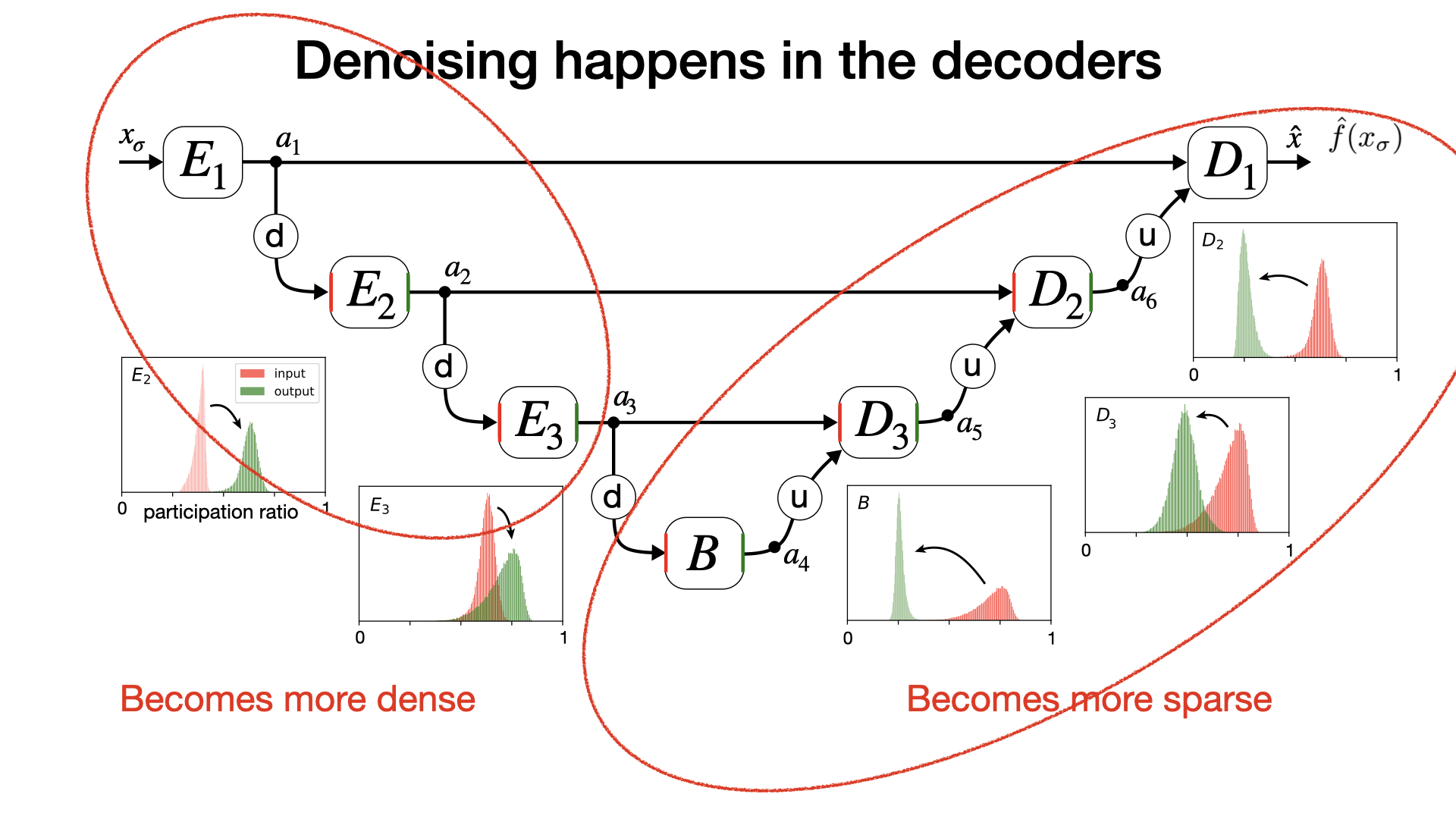
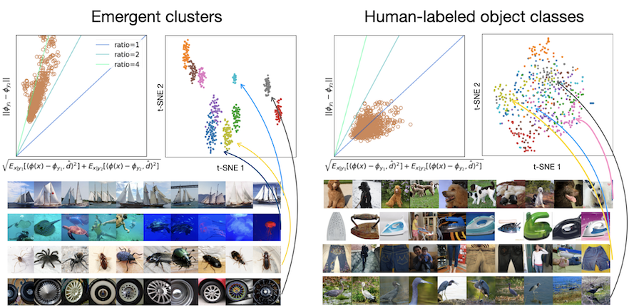
We also show the representation in the bottom block is most robust to noise level, so we focus on that in this paper. Take the vector of spatial averages of the channels in the last layer of the middle block. A k-means clustering of these vectors reveals that semantically similar images are near each other in this latent space: a fully-unsupervised bottom-up notion of similarity arises from the task of denoising (or noisy score estimation)! This notion of similarity is only partially aligned with object classes. For a model trained on ImageNet, Images within a cluster are visually similar and share global organization and semantic patterns, but they are not necessarily from the same class: dogs are clustered based on their pose, but not their breed. What is captures is “the gist of a scene.” [Oliva 2005]
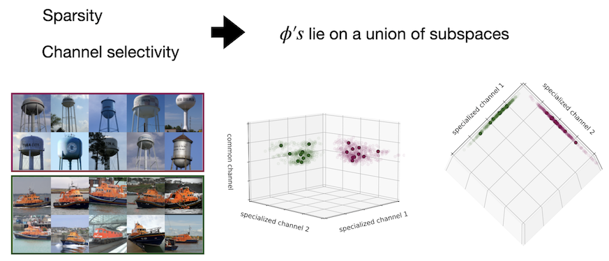
Two intriguing properties of the latent space are: the representation is sparse (most channels are off for a given image) and selective (a different subset of channels is activated for different images). A direct consequence of these properties is that the representation lies on a union of low-dimensional subspaces. From a geometric point of view: the denoising objective alone transforms a union of manifolds in the pixel space to a union of subspaces in the latent space. Within each subspace lies a cluster of image representations that are semantically similar.
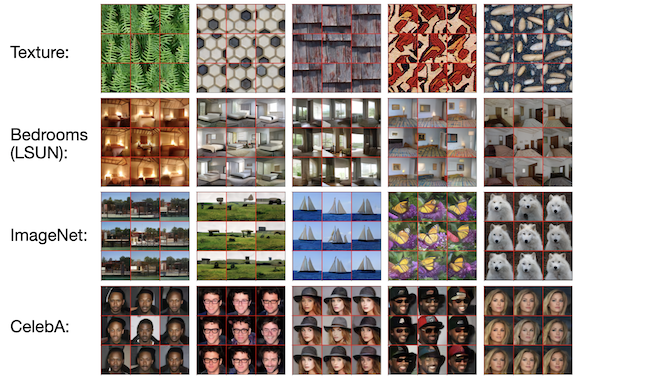
We further study this representation using a stochastic reconstruction algorithm: We sample from the density learned by the model while conditioning the trajectory on the model’s own representation of a target image. The algorithm alternates between a score step and a guidance step which matches the representation of the sample to that of the target. For a given target image, this algorithm generates samples that are similar to the target in the global features but different from it in location-non specific details. Some examples (each group shows 8 samples generated with internal representation matched to the (center) target image)
Reference: ZK, Mallat, Simoncelli, Unconditional CNN denoiser contain sparse semantic representations of images. arXiv, 2025.
PDF
Utilizing Learned Density Models to Solve Inverse Problems
Ultimately, we want “good” density models of images in order to use it real-world problems. From a Bayesian perspective, many problems in image processing and computer vision rely on having access to a density. In the era of deep learning, we can learn very powerful priors from data, through denoising, which opens the door to solving inverse problems with unprecedented quality.
Stochastic solutions to linear inverse problems using diffusion models
In the paper below, we introduced an algorithm to solve any linear inverse problem by sampling from a posterior. The posterior is built by combining the prior implicit in a denoiser and the likelihood function which returns partial meaurement of an image. Examples are low resolution image, missing pixels, blurred image, etc. The advantage of Bayesian approach is its universality. Once you have a “good” prior, you can utilize it to solve any inverse problems. This paper shortly preceded the wave of “diffusion models”, so the phrase does not apprear in the title, but variations of the algorithm emerged in the lietrature under the umberela of solving inverse problems using diffusion models…
Click here to see a summary
Reference:
ZK & Simoncelli, Solving linear inverse problems using the prior implicit in a denoiser. arXiv, July 2020. PDF | Project page
Later published as: ZK & Simoncelli, Stochastic Solutions for Linear Inverse Problems using the Prior Implicit in a Denoiser. NeurIPS, 2021. PDF
Learning optimal linear measurements for a prior embeded in a denoiser
Click here to see a summary
Zhang, ZK, Simoncelli, Brainard, Generalized Compressed Sensing for Image Reconstruction with Diffusion Probabilistic Models. TMLR, 2025 (J2C ICLR2026) PDF | Project page